Using RxInfer.jl to implement variational message passing on triplet Markov chains

The problem

In the previous post we introduced the concept of triplet Markov chains. However we are considering these models for a fixed observation vector \(\hat{\textbf{y}} = (\hat{y}_t)_{t=1}^T\).

Instead of a discrete inhomogeneous pairwise Markov model with a distribution \(p_p\) we will consider a simple inhomogeneous hidden Markov model (HMM). This is due to the fact that with the VMP constraint we can look at a dictionary \(\mathcal{W} = \mathcal{U} \times \mathcal{X}\) without any loss of generality and the corresponding distribution

\[p(\textbf{w}, \textbf{y}) = \pi(w_1) \prod_{t=2}^T p(w_t | w_{t-1}) \prod_{t=1}^T p(\hat{y}_t | w_t),\]

where \(y_t \sim \mathcal{N}(x_t, \sigma )\) and instead of minimising the KL divergence

\[\min_{q \in Q} D_{\text{KL}} \left[ q \| p_p \right]\]

in this post we are instead looking at an equivalent problem of maximising the ELBO

\[\max_{q \in Q} -D_{\text{KL}} \left[ q(\textbf{w}) \| p(\textbf{w}, \hat{\textbf{y}}) \right].\]

The advantage of this approach is that we don’t have to find the inhomogeneous tranisition matrix while getting the same solution \(q\). Let us recall that we defined the constraint for the variational message passing algorithm as

\[Q = \{ q | q(\textbf{w}) = \prod_{t=1}^T q_t(w_t) \}.\]

Defining the model in RxInfer.jl

The wonderful RxInfer tutorials have dealt with more difficult problems of inferring \(q\) where the transition distribution is not assumed to be fixed. This leads to the usage of DiscreteTransition node and Dirichlet distributions. This, I think, can’t be used directly to solve our problem of finding \(q \in Q\) in Triplet Markov Models.

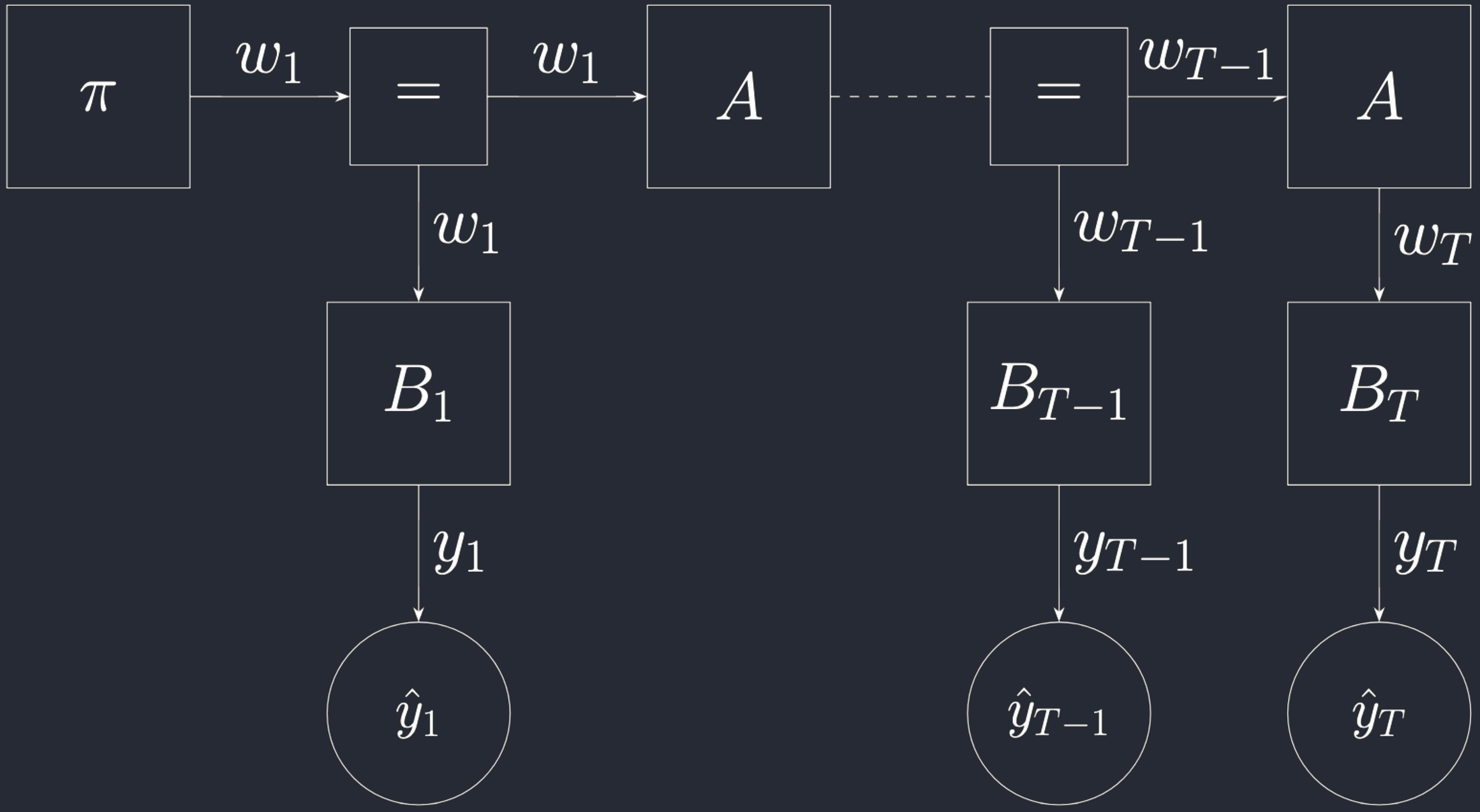
So we will define two custom nodes that will help us define a model in RxInfer. This post might cover the easiest use case in RxInfer yet. Below is the Forney-style Factor Graph for the model in question.

The general model without the custom node definitions can be defined in Julia.

import RxInfer

struct MetaTransition
    mat :: Matrix{Float64}
end

@model function hidden_markov_model(y)
    w[1] ~ Categorical(p1)
    y[1] ~ EmissionNode(w[1])
    for t in 2:length(y)
        w[t] ~ HmmTransition(w[t-1]) where { meta = MetaTransition(pt) }
        y[t] ~ EmissionNode(w[t])
    end
end

constraints = @constraints begin
    q(w) = q(w[begin])..q(w[end])
end

We write initial distribution vector, transition matrix and emission vector at timestep \(t\) as

\[\pi = (\pi_j)_{j=1}^{\\|\mathcal{W}\\|}\] \[A = \{a_{jj'} \\| a_{jj'} = p(w_t = j \\| w_{t-1} = j')\}\] \[B_t = \{b_j \\| b_j = p(y_t \\| w_t = j) \}.\]

It might be worth noting that \(B_t\) does not generally sum to one, but can be normalised.

Defining the custom nodes

Reading the documentation can help us define the custom nodes HmmTransition and EmissionNode. We will need to define the update rules and the average energy. Due to the constraints, the joint marginals need not be defined.

Transition node

Let us recall from the previous post that the optimal update rule is

\[q_t^{(1)}(w_t) = \frac{1}{Z_t} \exp \left[ \sum_{w_{t-1} } q_{t-1}^{(0)} (w_{t-1}) \ln p(w_t | w_{t-1}) \right]\] \[+ \frac{1}{Z_t} \exp \left[ \sum_{w_{t+1} } q_{t+1}^{(0)}(w_{t+1}) \ln p(w_{t+1} | u_t, x_t) \right].\]

Let us write this instead as \(q_t^{(1)}(w_t) \propto \nu_t^{\text{f}}(w_t) \nu_t^{\text{b}}(w_t),\) where the f denotes the forward component (summation over \(w_{t-1}\)) and b denotes the backward component (summing over \(w_{t+1}\)). To define a node, we need to specify at a timestep \(t\) the messages to the edge \(w_{t-1}\) and \(w_t\), denoted in Julia code as \(w_p\) and \(w_t\) respectively.

Let us write \(q_{t-1} = \text{Cat}(F)\) and \(q_{t} = \text{Cat}(G)\). Then we can write the messages as \(\ln \nu_t^{\text{f}} = \ln A \times F\) and \(\ln \nu_t^{\text{b}} = (\ln A)^T \times H\). We can now specify the messages in code.

@node HmmTransition Stochastic [wt, wp]

@rule HmmTransition(:wp, Marginalisation) (q_wt :: Categorical, meta::MetaTransition) = begin
    G = q_wt.p
    A = meta.mat
    ηs = exp.(log.(A)' * G)
    νs = ηs ./ sum(ηs)
    return Categorical(νs...)
end
@rule HmmTransition(:wt, Marginalisation) (q_wp :: Categorical, meta::MetaTransition) = begin
    F = q_wp.p
    A = meta.mat 
    ηs = exp.(log.(A) * F)  
    νs = ηs ./ sum(ηs)
    return Categorical(νs...)
end
@average_energy HmmTransition (q_wt::Categorical, q_wp::Categorical, meta::MetaTransition) = begin
    A = meta.mat
    G, F = q_wp.p, q_wt.p
    F' * log.(A) * G
end

The average energy here for node \(A\) and time \(t\) is simply

\[-E_{q_{t-1}(w_{t-1}) q_t(w_t)} \left[ \ln p(w_t \\| w_{t-1}) \right].\]

Emission node

For the emission node the definition is simpler as we are using clamped \(\hat{\textbf{y}}\) values. We need to define the average energy and the message to \(w_t\).