Multilevel Regression and Poststratification via Message Passing

Multilevel Regression and Poststratification via Message Passing

Reproducing the election turnout model from Gelman & Ghitza (2013) using variational message passing (RxInfer) instead of MCMC.

Setup

Voters are grouped into $J = J_1 \times J_2 \times J_3 = 5 \times 4 \times 51 = 1020$ cells defined by three demographic/geographic factors:

Factor	Levels	Notation
Income	5	$j_1 \in {1,\dots,5}$
Ethnicity	4	$j_2 \in {1,\dots,4}$
State	51	$j_3 \in {1,\dots,51}$

J = (5, 4, 51)
n_cells = prod(J)  # 1020

Terminology

A fixed effect is a regression coefficient that is the same for every observation. It captures the average relationship between a covariate and the outcome across the entire population. In this model the fixed effects are $\beta_0, \beta_{\text{inc}}, \beta_{\text{rep}}, \beta_{\text{stateinc}}$ – one scalar each, shared by all 1020 cells.

A random effect is a coefficient that varies across groups and is itself modelled as drawn from a distribution (typically Gaussian). Rather than estimating a completely separate parameter per group, the shared distribution pools information across groups, shrinking noisy estimates toward the group mean. In this model the random effects are $\alpha^{\text{inc}}_{j_1}$, $\alpha^{\text{eth}}_{j_2}$, and $\alpha^{\text{state}}_{j_3}$ – one per level of each grouping factor, drawn from $\mathcal{N}(0, \sigma^2_{\text{group}})$.

The distinction matters for the prior: fixed effects get a vague prior (large variance), while random effects get a tighter prior (smaller variance) that regularises groups with little data toward zero.

Generative process

Each cell $j = (j_1, j_2, j_3)$ has a covariate row $\mathbf{x}_j \in \mathbb{R}^{p}$ and an observed turnout count $y_j$.

Covariates

The design matrix $\mathbf{X} \in \mathbb{R}^{J \times p}$ with $p = 64$ is composed of:

\[\mathbf{x}_j = \bigl[\underbrace{1,\; \text{inc}_{j_1},\; \text{repvote}_{j_3},\; \text{stateinc}_{j_3}}_{\text{fixed effects (4)}},\; \underbrace{\mathbf{e}_{j_1}^{(5)}}_{\text{income RE}},\; \underbrace{\mathbf{e}_{j_2}^{(4)}}_{\text{ethnicity RE}},\; \underbrace{\mathbf{e}_{j_3}^{(51)}}_{\text{state RE}}\bigr]\]

where $\mathbf{e}_{k}^{(L)}$ is the $k$-th standard basis vector in $\mathbb{R}^L$ (one-hot encoding). The fixed-effect covariates and group dummies are assembled per cell:

n_params = n_fixed + J[1] + J[2] + J[3]  # 4 + 5 + 4 + 51 = 64
X = zeros(n_cells, n_params)

for j in CartesianIndices(J)
    idx = LinearIndices(zeros(J))[j]
    inc, eth, state = Tuple(j)

    # Fixed effects columns
    X[idx, 1] = 1.0                              # intercept
    X[idx, 2] = income_levels[inc]                # income level
    X[idx, 3] = state_covariates[state, 1]        # prev rep vote
    X[idx, 4] = state_covariates[state, 2]        # state income

    # One-hot dummies for group-level random effects
    X[idx, n_fixed + inc] = 1.0                   # income group
    X[idx, n_fixed + J[1] + eth] = 1.0            # ethnicity group
    X[idx, n_fixed + J[1] + J[2] + state] = 1.0   # state group
end

Cell sizes

The number of eligible voters per cell is drawn uniformly:

\[N_j \sim \text{Uniform}(40{,}000,\; 160{,}000)\]

Linear predictor

The combined parameter vector $\boldsymbol{\beta} \in \mathbb{R}^{64}$ stacks all effects:

\[\boldsymbol{\beta} = \begin{pmatrix} \beta_0 \\ \beta_{\text{inc}} \\ \beta_{\text{rep}} \\ \beta_{\text{stateinc}} \\ \alpha^{\text{inc}}_1, \dots, \alpha^{\text{inc}}_5 \\ \alpha^{\text{eth}}_1, \dots, \alpha^{\text{eth}}_4 \\ \alpha^{\text{state}}_1, \dots, \alpha^{\text{state}}_{51} \end{pmatrix}\]

so the logit of the turnout probability in cell $j$ is:

\[\text{logit}(\theta_j) = \mathbf{x}_j^\top \boldsymbol{\beta} = \underbrace{\beta_0 + \beta_{\text{inc}} \cdot \text{inc}_{j_1} + \beta_{\text{rep}} \cdot \text{repvote}_{j_3} + \beta_{\text{stateinc}} \cdot \text{stateinc}_{j_3}}_{\text{fixed effects}} + \underbrace{\alpha^{\text{inc}}_{j_1} + \alpha^{\text{eth}}_{j_2} + \alpha^{\text{state}}_{j_3}}_{\text{random effects}}\]

logits = X * beta_expanded_true
prob = 1 ./ (1 .+ exp.(-logits))
y = [rand(rng, Binomial(N[j], prob[j])) for j in 1:n_cells]

Likelihood

\[y_j \mid \theta_j \sim \text{Binomial}(N_j,\; \theta_j), \qquad \theta_j = \text{logistic}(\mathbf{x}_j^\top \boldsymbol{\beta})\]

True parameter values

Parameter	Value
$\beta_0$ (intercept)	$0.5$
$\beta_{\text{inc}}$ (income level)	$-0.05$
$\beta_{\text{rep}}$ (prev. Republican vote share)	$1.0$
$\beta_{\text{stateinc}}$ (state income)	$-8 \times 10^{-7}$
$\alpha^{\text{inc}}_k$	$\sim \mathcal{N}(0,\; 0.3^2)$
$\alpha^{\text{eth}}_k$	$\sim \mathcal{N}(0,\; 0.3^2)$
$\alpha^{\text{state}}_k$	$\sim \mathcal{N}(0,\; 0.5^2)$

Inference model

Prior

The prior on $\boldsymbol{\beta}$ encodes the hierarchical structure through a block-diagonal covariance:

\[\boldsymbol{\beta} \sim \mathcal{N}\!\left(\mathbf{0},\; \boldsymbol{\Sigma}_0\right), \qquad \boldsymbol{\Sigma}_0 = \text{diag}\!\left(\underbrace{100, 100, 100, 100}_{\text{fixed effects}},\; \underbrace{1, \dots, 1}_{5\text{ income}},\; \underbrace{1, \dots, 1}_{4\text{ ethnicity}},\; \underbrace{1, \dots, 1}_{51\text{ state}}\right)\]

The large variance ($100$) on fixed effects encodes a vague prior. The unit variance on random effects acts as a Gaussian shrinkage prior, playing the role of the hierarchical variance component $\sigma^2_\alpha$ in the original Gelman specification. These variances can be fixed (as in this simple example) or estimated from data via variational EM (see “Hierarchical variance estimation” below).

prior_var = zeros(n_params)
prior_var[1:n_fixed] .= 100.0                          # fixed effects
prior_var[n_fixed+1:n_fixed+J[1]] .= 1.0               # income RE
prior_var[n_fixed+J[1]+1:n_fixed+J[1]+J[2]] .= 1.0     # ethnicity RE
prior_var[n_fixed+J[1]+J[2]+1:end] .= 1.0              # state RE
prior_cov = diagm(prior_var)

Likelihood (Polya-Gamma augmentation)

The logistic-binomial likelihood is not conjugate with Gaussian messages. Naively, the posterior

\[p(\boldsymbol{\beta} \mid \mathbf{y}) \propto p(\boldsymbol{\beta}) \prod_{j=1}^{J} \frac{\binom{N_j}{y_j} \exp(y_j \cdot \mathbf{x}_j^\top \boldsymbol{\beta})}{(1 + \exp(\mathbf{x}_j^\top \boldsymbol{\beta}))^{N_j}}\]

has no closed-form normalising constant. Polson, Scott & Windle (2013) showed that by introducing auxiliary Polya-Gamma variables $\omega_j$ the logistic factor can be written as a Gaussian integral (Gundersen 2019):

\[\frac{(e^\psi)^a}{(1+e^\psi)^b} = 2^{-b} e^{\kappa \psi} \int_0^\infty e^{-\omega \psi^2 / 2}\; p(\omega)\, d\omega, \qquad \omega \sim \text{PG}(b,\, 0)\]

where $\kappa = a - b/2$. Conditioning on $\omega_j$ turns each likelihood factor into a Gaussian observation on $\psi_j = \mathbf{x}_j^\top \boldsymbol{\beta}$:

\[\psi_j \mid \omega_j \;\sim\; \mathcal{N}\!\left(\frac{\kappa_j}{\omega_j},\; \frac{1}{\omega_j}\right), \qquad \omega_j \mid \psi_j \;\sim\; \text{PG}(N_j,\; \psi_j)\]

RxInfer’s BinomialPolya node implements this augmentation as a message-passing primitive. By default it evaluates the analytical expectation of the Polya-Gamma auxiliary variable using the closed-form expression $\mathbb{E}[\omega] = \frac{b}{2c}\tanh\left(\frac{c}{2}\right)$ (via mean(PolyaGammaHybridSampler(b, c)) from PolyaGammaHybridSamplers.jl) and sends a Gaussian message back to $\boldsymbol{\beta}$. Alternatively, when BinomialPolyaMeta is provided, the node draws Monte Carlo samples from $\text{PG}(N_j, \mathbf{x}_j^\top\boldsymbol{\beta})$ using rand() and averages them. The default analytical mode is deterministic and sufficient when the current estimate of $\mathbf{x}_j^\top\boldsymbol{\beta}$ is a reasonable point around which to linearise.

@model function mrp_model(x, n, y, prior_cov)
    beta ~ MvNormal(mean = zeros(n_params), cov = prior_cov)
    for j in eachindex(y)
        y[j] ~ BinomialPolya(x[j], n[j], beta) where {
            dependencies = RequireMessageFunctionalDependencies(
                beta = MvNormal(zeros(n_params), diageye(n_params))
            )
        }
    end
end

The RequireMessageFunctionalDependencies annotation provides an initial message for $\boldsymbol{\beta}$ to break the circular dependency at the first iteration.

Message passing

Inference proceeds by iterating variational messages on the factor graph:

\[\underbrace{\mathcal{N}(\boldsymbol{\beta} \mid \mathbf{0}, \boldsymbol{\Sigma}_0)}_{\text{prior}} \longrightarrow \boldsymbol{\beta} \longleftarrow \prod_{j=1}^{1020} \underbrace{f_{\text{BinomialPolya}}(y_j,\, \mathbf{x}_j,\, N_j,\, \boldsymbol{\beta})}_{\text{likelihood factors}}\]

At each iteration, every BinomialPolya factor:

1. Receives the current posterior approximation $q^{(t)}(\boldsymbol{\beta})$
2. Computes $\mathbb{E}[\omega_j]$ under $\text{PG}(N_j,\; \mathbf{x}_j^\top \boldsymbol{\mu}^{(t)})$
3. Sends a Gaussian message $\mathcal{N}^{-1}(\boldsymbol{\xi}_j,\; \boldsymbol{\Lambda}_j)$ back to $\boldsymbol{\beta}$, where $\boldsymbol{\Lambda}_j = \mathbb{E}[\omega_j]\, \mathbf{x}_j \mathbf{x}_j^\top$ and $\boldsymbol{\xi}_j = \kappa_j\, \mathbf{x}_j$

The prior and all 1020 likelihood messages are combined in natural-parameter form:

\[\boldsymbol{\Lambda}_q = \boldsymbol{\Sigma}_0^{-1} + \sum_{j=1}^{J} \boldsymbol{\Lambda}_j, \qquad \boldsymbol{\xi}_q = \boldsymbol{\Sigma}_0^{-1}\mathbf{0} + \sum_{j=1}^{J} \boldsymbol{\xi}_j\]

After convergence the posterior is Gaussian:

\[q(\boldsymbol{\beta}) = \mathcal{N}(\boldsymbol{\beta} \mid \boldsymbol{\mu}_q, \boldsymbol{\Sigma}_q), \qquad \boldsymbol{\Sigma}_q = \boldsymbol{\Lambda}_q^{-1}, \quad \boldsymbol{\mu}_q = \boldsymbol{\Sigma}_q \boldsymbol{\xi}_q\]

results = infer(
    model = mrp_model(prior_cov = prior_cov),
    data = (x = x_data, n = n_data, y = y),
    iterations = 20,
    returnvars = KeepLast(),
    free_energy = true,
)

Predictions

The posterior mean turnout probability for cell $j$:

\[\hat{\theta}_j = \text{logistic}\!\left(\mathbf{x}_j^\top \boldsymbol{\mu}_q\right)\]

prob_pred = [1 / (1 + exp(-dot(x_data[j], beta_post))) for j in 1:n_cells]

Comparison with MCMC

The standard approach to this model is Markov chain Monte Carlo, typically a Polya-Gamma Gibbs sampler (Polson et al. 2013) or Hamiltonian Monte Carlo as implemented in Stan. The message-passing approach above differs in several ways.

What MCMC gives you

MCMC targets the exact posterior $p(\boldsymbol{\beta} \mid \mathbf{y})$. Given enough samples it can represent arbitrary posterior shapes – multimodality, skewness, heavy tails. A Polya-Gamma Gibbs sampler for this model alternates between:

\[\omega_j \mid \boldsymbol{\beta} \sim \text{PG}(N_j,\; \mathbf{x}_j^\top \boldsymbol{\beta}), \qquad j = 1, \dots, J\] \[\boldsymbol{\beta} \mid \boldsymbol{\omega} \sim \mathcal{N}(\boldsymbol{\mu}_\omega,\; \boldsymbol{\Sigma}_\omega)\]

where $\boldsymbol{\Sigma}_\omega = (\mathbf{X}^\top \boldsymbol{\Omega} \mathbf{X} + \boldsymbol{\Sigma}_0^{-1})^{-1}$ and $\boldsymbol{\mu}_\omega = \boldsymbol{\Sigma}_\omega (\mathbf{X}^\top \boldsymbol{\kappa} + \boldsymbol{\Sigma}_0^{-1} \boldsymbol{\mu}_0)$, with $\boldsymbol{\Omega} = \text{diag}(\omega_1, \dots, \omega_J)$ and $\kappa_j = y_j - N_j / 2$ (Gundersen 2019).

Each Gibbs sweep requires sampling $J$ Polya-Gamma variables and solving a $p \times p$ linear system. After a burn-in period, the chain provides correlated draws from the true posterior. Convergence diagnostics ($\hat{R}$, effective sample size) are needed to assess whether the chain has mixed.

What message passing gives you

Variational message passing returns a Gaussian approximation $q(\boldsymbol{\beta}) = \mathcal{N}(\boldsymbol{\mu}_q, \boldsymbol{\Sigma}_q)$ that minimises the KL divergence $\text{KL}(q | p(\cdot \mid \mathbf{y}))$. This is a structured optimisation, not a stochastic simulation. The algorithm:

• Has a deterministic convergence criterion (Bethe free energy), rather than stochastic diagnostics
• Converges in a fixed, small number of iterations (20 in this model) rather than requiring thousands of samples plus burn-in
• Produces a closed-form posterior (mean and covariance matrix) rather than a bag of samples that must be stored and post-processed
• Uses the same Polya-Gamma identity as the Gibbs sampler internally, but takes expectations $\mathbb{E}[\omega_j]$ instead of drawing samples

The trade-off

	Message passing	MCMC
Output	$\mathcal{N}(\boldsymbol{\mu}_q, \boldsymbol{\Sigma}_q)$ (parametric)	Samples from $p(\boldsymbol{\beta} \mid \mathbf{y})$ (nonparametric)
Posterior shape	Gaussian (unimodal, symmetric)	Arbitrary
Cost per iteration	$O(Jp^2)$ deterministic	$O(Jp^2)$ + PG sampling + mixing time
Total cost	Fixed iterations to convergence	Burn-in + effective samples / autocorrelation
Convergence check	Free energy (deterministic)	$\hat{R}$, ESS (stochastic)
Uncertainty calibration	Tends to underestimate variance	Asymptotically exact
Streaming data	Natural (update messages incrementally)	Restart chain or use sequential Monte Carlo

When message passing makes more sense

• Large-scale or streaming settings. With 1020 cells and 64 parameters, message passing converges in 20 deterministic iterations. An MCMC sampler would require tuning the number of samples, diagnosing mixing across all 64 dimensions, and storing thousands of posterior draws. As $J$ grows to tens of thousands of cells (e.g. finer demographic stratification), the gap widens.

• Repeated inference. If the model is re-fit regularly as new polling data arrives (e.g. nightly election tracking), a deterministic algorithm with predictable runtime is easier to deploy than a sampler whose wall-clock time depends on mixing.

• When the posterior is well-approximated by a Gaussian. For logistic regression with many observations per parameter, the Bernstein-von Mises theorem guarantees the posterior concentrates toward a Gaussian. With $\sim 100{,}000$ voters per cell, this model is firmly in this regime. The Gaussian approximation is tight, and the extra fidelity of MCMC buys little.

When MCMC makes more sense

• Few observations, strong prior-data conflict, or multimodal posteriors. A Gaussian approximation can miss important posterior structure when data is sparse or the model is weakly identified.

• Posterior functionals. If the quantity of interest is a nonlinear function of $\boldsymbol{\beta}$ (e.g. the probability that a specific state flips), MCMC samples can be transformed directly. A Gaussian approximation requires either the delta method or additional sampling from $q$.

Extensions: full Gelman & Ghitza model

The simple model above demonstrates the basic design-matrix approach with random intercepts. The full Gelman & Ghitza (2013) model adds several additional structures, all representable within the same expanded design matrix framework.

Fixed interactions

Interaction terms between continuous covariates are pre-computed and added as additional fixed-effect columns. For example, the turnout model includes $\texttt{z_inc} \times \texttt{z_incstt}$ and $\texttt{z_inc} \times \texttt{z_trnprv}$:

\[\mathbf{x}_j = \bigl[\dots,\; \underbrace{x_{\text{inc}} \cdot x_{\text{incstt}}}_{\text{interaction}},\; \underbrace{x_{\text{inc}} \cdot x_{\text{trnprv}}}_{\text{interaction}},\; \dots\bigr]\]

These columns receive the same vague prior variance ($100$) as other fixed effects.

Random slopes

A random slope (z_inc | stt) allows the effect of income to vary by state. In the design matrix, this is encoded as covariate-weighted dummies: for each state $s$, the slope column contains z_inc$_{j}$ if observation $j$ belongs to state $s$, and $0$ otherwise:

\[X_{j, \text{slope}_s} = \begin{cases} \texttt{z\_inc}_j & \text{if } \text{stt}_j = s \\ 0 & \text{otherwise} \end{cases}\]

This creates a separate block of $K_s$ columns per group, with the same group-level shrinkage prior as the corresponding random intercepts.

Two-way interaction random effects

Cross-group random effects like $(1 \mid \texttt{stt:eth})$ are encoded as one-hot dummies for each unique combination. With 51 states and 4 ethnicities, this produces $51 \times 4 = 204$ dummy columns. The full model includes 9 such pairs:

Interaction	Levels
reg_eth	$5 \times 4 = 20$
reg_inc	$5 \times 5 = 25$
reg_age	$5 \times 4 = 20$
stt_eth	$51 \times 4 = 204$
stt_inc	$51 \times 5 = 255$
stt_age	$51 \times 4 = 204$
eth_inc	$4 \times 5 = 20$
eth_age	$4 \times 4 = 16$
inc_age	$5 \times 4 = 20$

Together with the intercept (1), 3 fixed effects, 2 fixed interactions, 5 main RE groups (69 levels), 4 slope groups (64 levels), and 9 interaction RE groups (784 levels), the full model has approximately 941 parameters.

Memory limitation with RxInfer

RxInfer’s factor graph stores a dense $p \times p$ covariance matrix per message, per observation node, in both directions. For the full 941-parameter model with $\sim 3000$ observed cells this requires roughly $3000 \times 2 \times 941^2 \times 8 \approx 40\;\text{GB}$ for messages alone, plus substantial reactive-graph overhead. This exceeds typical workstation memory.

In practice we run a medium model (~140 parameters) that includes all fixed effects, fixed interactions, main RE groups, and random slopes — but omits the 9 two-way interaction RE groups. This fits comfortably in $\sim 2\;\text{GB}$. To recover the full 941-parameter model one would need to bypass RxInfer’s factor graph and accumulate the natural-parameter Polya-Gamma messages manually in a single $p \times p$ matrix per iteration, reducing memory from $O(Jp^2)$ to $O(p^2)$.

Hierarchical variance estimation via variational EM

In the full Gelman specification, each random effect group $g$ has its own variance $\sigma^2_g$ with an $\text{Exponential}(1)$ prior (in PyMC) or $\text{Inv-}\chi^2$ prior (in classical formulation). Rather than fixing these in $\boldsymbol{\Sigma}_0$, we estimate them using variational EM.

The challenge is that BinomialPolya requires a Gaussian prior $\boldsymbol{\beta} \sim \mathcal{N}(\mathbf{0}, \boldsymbol{\Sigma}_0)$ with $\boldsymbol{\Sigma}_0$ fixed during message passing. The group-level variances sit outside this node. We therefore use a two-stage iterative procedure:

E-step (message passing): Fix $\boldsymbol{\Sigma}_0$, run BinomialPolya inference to obtain $q(\boldsymbol{\beta}) = \mathcal{N}(\boldsymbol{\mu}_q, \boldsymbol{\Sigma}_q)$.

M-step (update variances): For each random effect group $g$ with $K_g$ levels at column indices $\mathcal{I}_g$, update:

\[\hat{\sigma}^2_g = \frac{1}{K_g} \sum_{k \in \mathcal{I}_g} \left( \mu_{q,k}^2 + \Sigma_{q,kk} \right)\]

This is the expected variance under the posterior, accounting for posterior uncertainty in each coefficient. It is the standard variational EM update for variance components (see e.g. Beal 2003, §3.4).

Rebuild $\boldsymbol{\Sigma}_0$ with updated group variances and repeat.

function update_sigmas!(sigmas, mu_q, Sigma_q, col_ranges)
    for (name, rng) in col_ranges
        if startswith(String(name), "re_")
            K = length(rng)
            σ2 = sum(mu_q[rng].^2 .+ diag(Sigma_q)[rng]) / K
            sigmas[group_key] = sqrt(max(σ2, 1e-8))
        end
    end
end

This converges in 3–5 outer iterations. The estimated $\hat{\sigma}_g$ values are analogous to the posterior mean of $\sigma_g$ in the full Bayesian model. Groups with fewer data points or more homogeneous effects will have their variance shrunk toward zero, while well-identified groups retain larger variances.

Results

The medium model (139 parameters: intercept, 3 fixed effects, 2 fixed interactions, 5 main RE groups, 4 random slope groups) was fit for both turnout and vote choice in 2004 and 2008, then poststratified with census population weights and calibrated to known state-level totals.

National aggregates

	Turnout	Republican vote share
2004	0.584	0.402
2008	0.628	0.346
Swing	+3.6 pp	−4.9 pp

Figure 1: Income and vote choice by state (2008 whites)

Each line is one state; colour reflects 2008 Republican vote share (red = Republican, blue = Democratic). The varying-slope model captures the steeper income gradient in blue states (richer voters more Republican) versus the flatter gradient in red states.

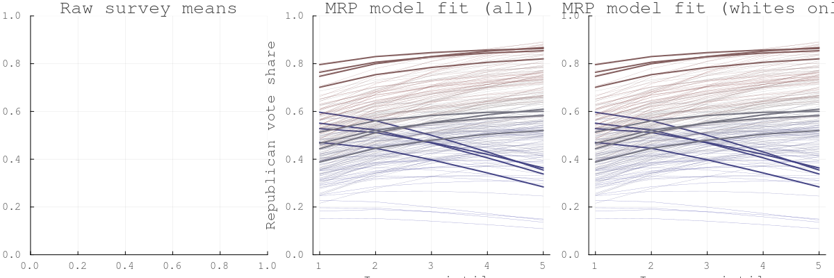
Figure 2: Per-state income panels

48 state panels sorted by Republican vote share (descending). Gray = all voters, orange = white voters. The income gradient in vote choice is visible across states, with white voters consistently more Republican.

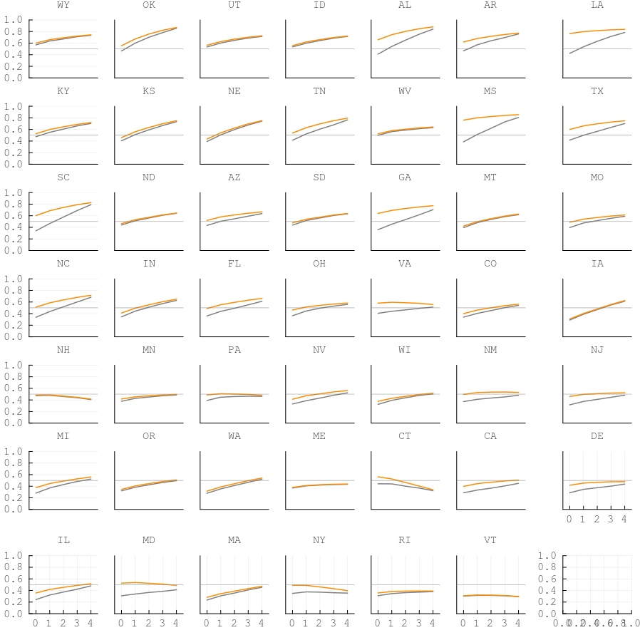
Figure 3: Bubble plots — turnout vs. vote choice at increasing granularity

Bubble size proportional to population. Colour by ethnicity: white, black, red (Hispanic), green (other). Left to right: state×ethnicity, state×ethnicity×income, full cells. Black voters cluster in the low-Republican/high-turnout quadrant.

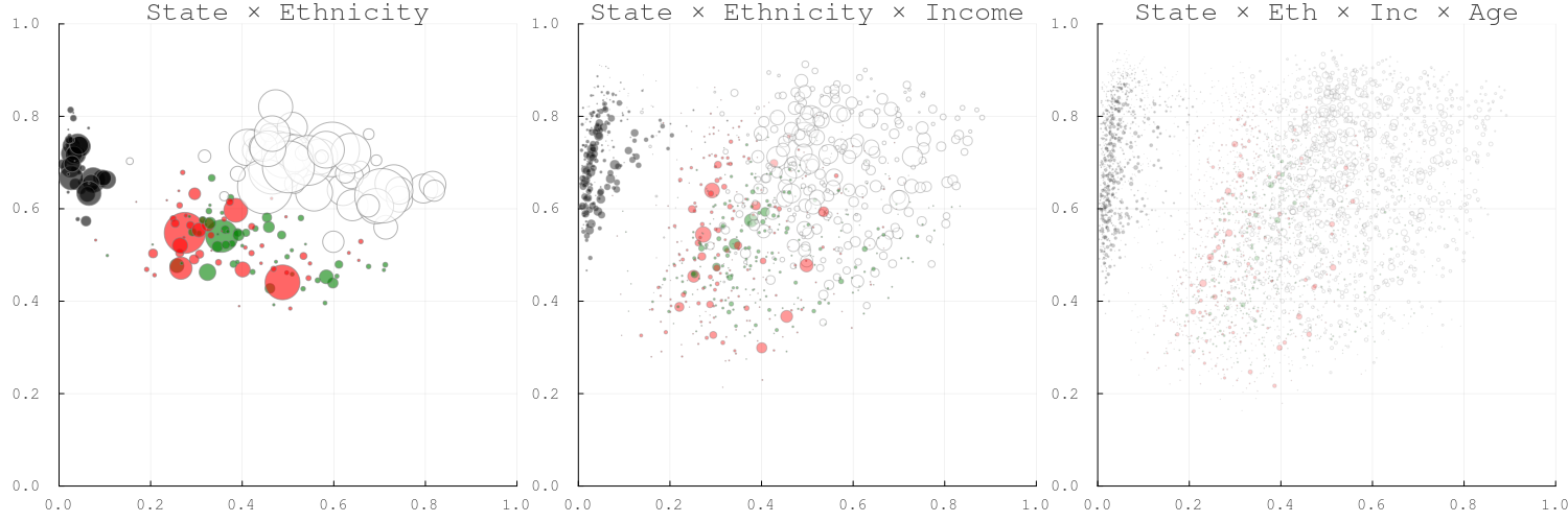
Figure 4: McCain swing by age and income among whites

Blue-white-red scale: blue = swing toward Obama, red = swing toward McCain. Each strip shows states ordered by index. Young and low-income white voters swung toward Obama; older and higher-income voters swung toward McCain.

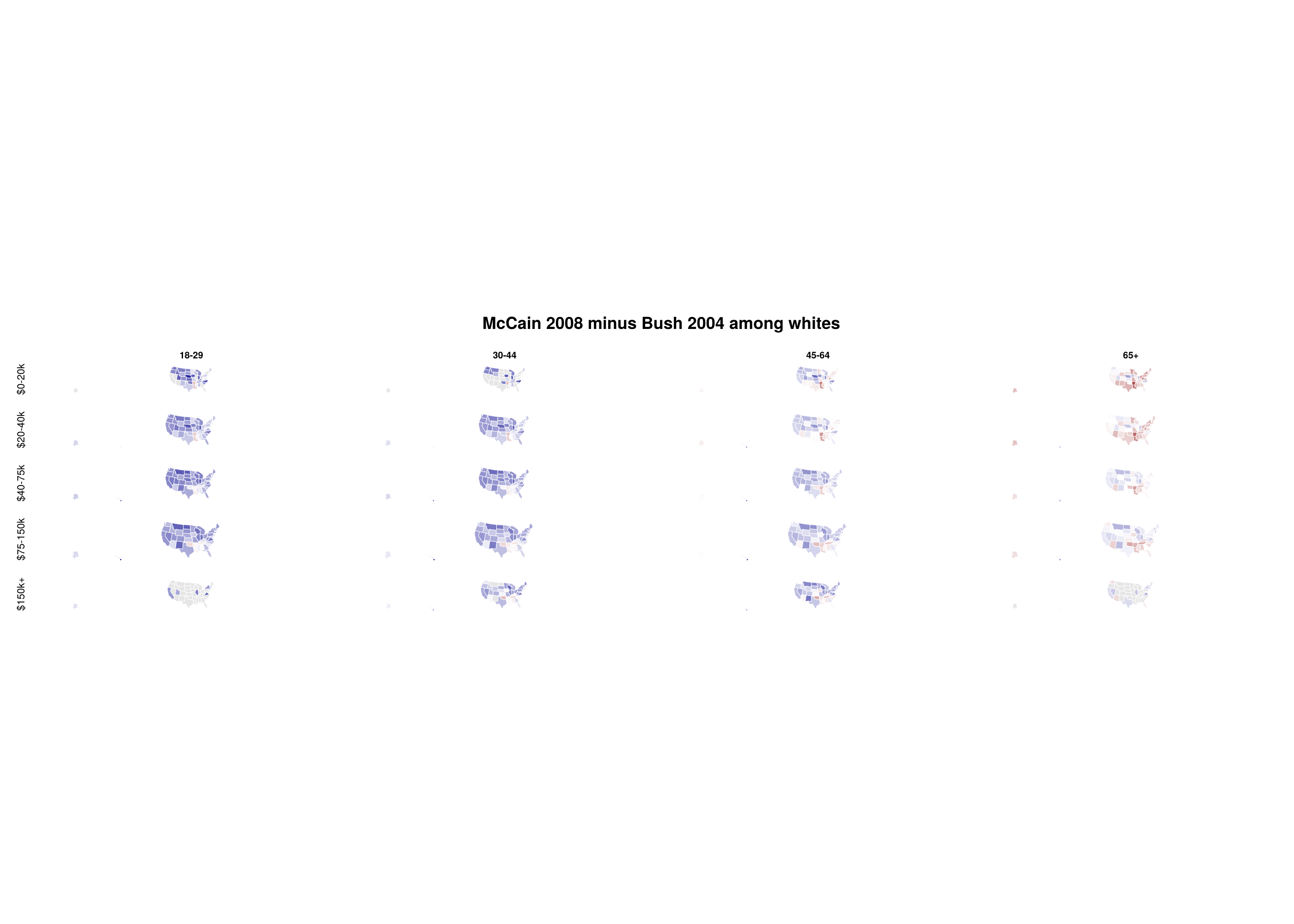
Figure 5: Turnout swing (2008 minus 2004) by ethnicity, age, and income

Bars show 2008 population share by income quintile; lines show turnout swing. Red dashed line = national aggregate swing. Blue-highlighted panels indicate groups with turnout swing above 5 pp. Black voters show the largest turnout increases across all age and income groups (Obama mobilisation effect).

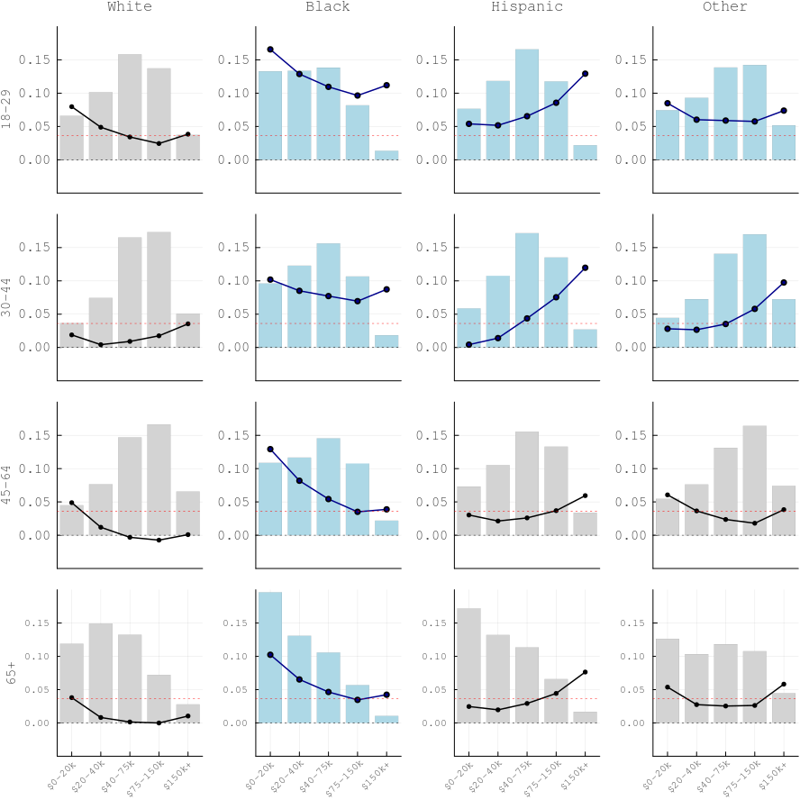
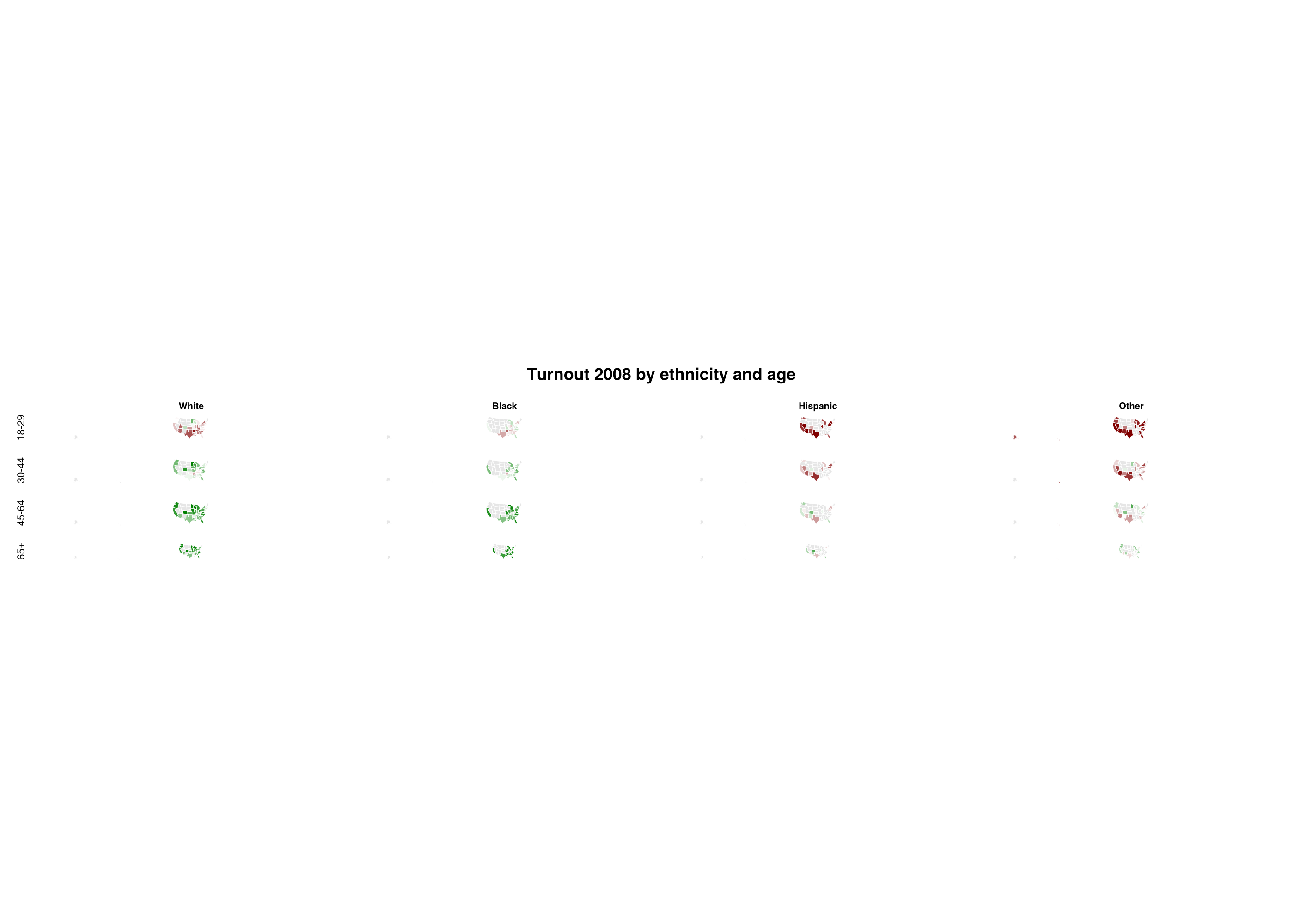
Figure 6: Turnout levels (2008) by ethnicity and age

Red-white-green scale: green = high turnout (≥0.8), red = low turnout (≤0.4). Each strip shows states. Older white voters have the highest turnout; young minorities the lowest. Small-population cells are masked out.